Synoptic summer surveys of food web biomass in the South Fork and Mainstem Eel River
This is a period of rapid and critical change for the Eel River ecosystem. Many groups are keeping their eyes on the Eel watershed, and we are grateful for their vigilance and their partnership. Here is what the Berkeley-based Eyes on the Eel group is doing:
We survey selected tributaries and mainstem reaches near their confluences within the S. Fork and mainstem Eel basins to document changes in key species and groups of organisms that make up the summer food web in these channels. We’re interested in what the food webs look like during three periods of summer baseflow: mid-June, when production of algae, invertebrates, and growth of fish is typically peaking; July, when temperatures are warmest; and September, when discharge is lowest.
______________________________________________________________________________________________________________________________________________________________________________________________

______________________________________________________________________________________________________________________________________________________________________________________________
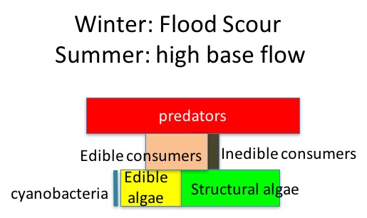
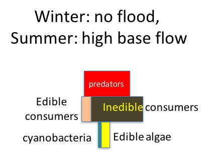
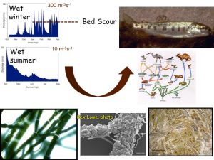
Our data could address a number of questions, but we are initially interested in testing hypotheses about “patterns of trophic level biomass” (the biomass of organisms in various feeding groups at different levels in food webs: basal (primary producer, mostly algae), intermediate (consumers, mostly aquatic invertebrates), and top (predators, mostly fish). Previous work at the Angelo Reserve suggested that year-to-year variation in food webs, particularly the peak abundance of attached algae, depends on whether or not scouring floods occurred during the previous winter. The dominant type of algae–i.e., the prevalence of nutritious diatoms versus potentially toxic cyanobacteria–depends on how much summer flows drop and temperatures warm. Different patterns of trophic level biomass are also expected in sunlit mainstem channels versus darker tributaries. Clearly, there will be changes over the summer season as well. Will patterns we’ve seen within the Angelo Reserve in the upper South Fork, where the river drains 116-160 km2, apply more broadly across the 9,540 km2 Eel River?
 Hypothesis I: Effect of annual hydrology


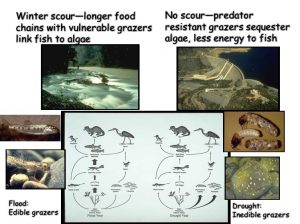
During the summer low flow season, we think the algal-based food web of the Eel River can assemble into one of three alternative states (Power et al. 2008, 2014, 2015). In Salmon state, rock substrates and streamers of the macroalga Cladophora glomerata become covered with nutritious diatoms, which in turn support many edible prey–largely primary consumers (invertebrates and tadpoles that eat living or dead plant tissue). Diatom energy, nutrients, and lipids (including critical polyunsaturated fatty acids, or PUFAs) are transferred up the food chain to support rearing juvenile salmonids and other predators. Salmon state generally occurs after winters when one or more bankfull floods scour out grazing insects that otherwise can grow large enough to escape gape-limited predators the next summer. These armored, predator-resistant but slow-growing grazers include stone-cased caddisflies: (Dicosmoecus in mainstems, and Glossosoma and Neophylax in both mainstems and tributaries). Dicosmoecus state characterizes summer food webs that follow winters when scouring winter floods have not occurred. In Dicosmoecus state, large macroalgal blooms do not proliferate because these large armored grazers are very abundant the following summer, and graze down the algae before it can grow long streamers. Algal energy and nutrients is sequestered in the body of large armored (or sessile) grazers that aren’t vulnerable to juvenile salmonids, so they don’t grow as well. In recent years, a third summer food web state, Cyanobacteria state, has emerged. Potentially neurotoxic cyanobacteria (Anabaena spp.) can proliferate if summer base flows grow critically low, so that sunny mainstems warm and backwaters or side pools stagnate. Blankets of cyanobacteria can overgrow the edible diatom epiphytes and their green macroalgal hosts, forming what Keith Bouma-Gregson calls “spires”. Bouma-Gregson et al., 2017 Other neurotoxic cyanobacteria (Phormidium spp, Bouma-Gregson et al. in prep) have been observed attached to rocks in tributary mainstem riffles where flows remain relatively strong. It is possible that they become public health threats after they detach and accumulate in backwater areas (Bouma-Gregson, pers comm.).
These three proposed food web “states” are simplified hypotheses, and in need of constant tests for better understanding. We need to learn more about the environmental conditions that steer the river food web towards one state or another to forecast summer food web structure in the Eel and manage flows and land cover for food webs that support salmonids.
______________________________________________________________________________________________________________________________________________________________________________________________
Hypothesis II: Downstream changes in food web controls
Food web assembly is controlled less by energy loading and more by disturbance regime as one moves downstream into habitats with increasing sunlight and bedload mobility (decreasing substrate stability (Finlay et al. 2010; Power, Kupferberg, Cooper and Deas, 2015 ). We expect that tributaries will buffer river networks against some of the severe low-flow changes we anticipate in mainstem channels (Uno and Power 2014).
Hypothesis III: Critical flow thresholds
Summertime water extraction can potentially tip the Eel food web from salmon-supporting to cyanobacterialy degraded states (Bauer et al. 2015; Carah et al., 2015, Power et al. 2015).
______________________________________________________________________________________________________________________________________________________________________________________________
Methods
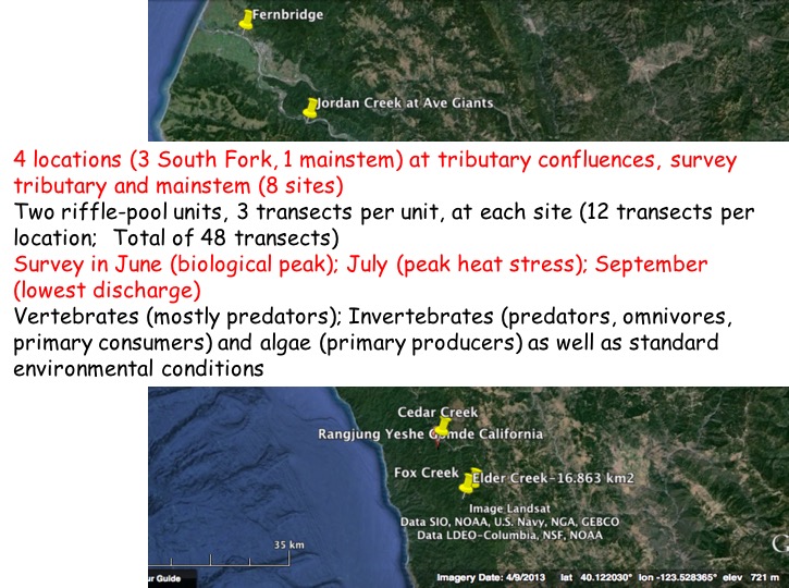 We selected four tributary-mainstem confluences, one in the mainstem Eel at Jordan Creek, and three in the South Fork. We also have some infrequently monitored transects ~100 m upstream from the Fernbridge, near the Eel estuary. We have monitored now in 2015, 2016, and 2017 (but started in July in 2015).
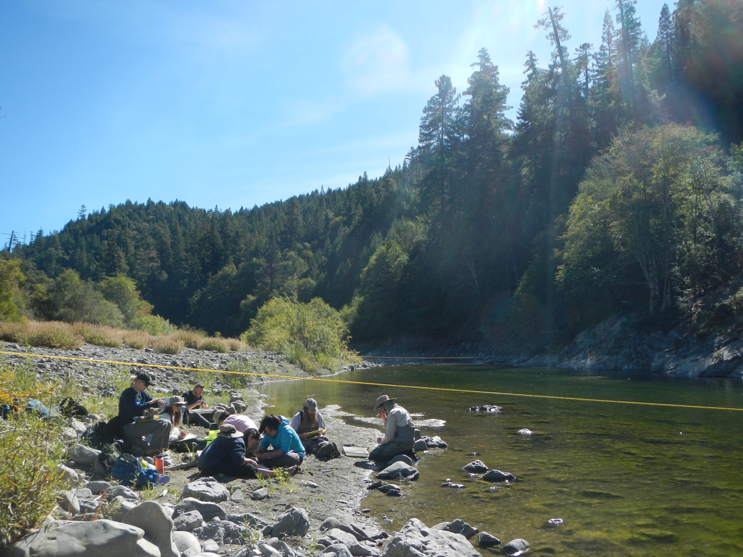
With a team of 10-12, we can complete a site (one mainstem and its tributary) in one day, so each complete survey takes 4 days in our June, July or September sampling effort.
Initial set up–site benchmarks and mapping:
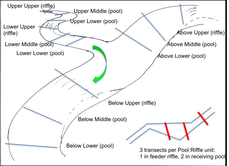
 At a given site (mainstem-tributary confluence), we choose four ‘hydraulic units’ (a riffle and its receiving pool) on upstream and downstream reaches of the tributary, and above and below the confluence on the mainstem. Transect cross-sections, one across the upstream (riffle), and two across the pool, are benchmarked on both sides with small nails and tags in trees (or rock).
Surveys of biota and seasonal environmental conditions
 Snorkeling counts of large fish are done first so that large vertebrates won’t be scared away. One (in small tributaries) or two (in wider mainstems) snorkelers (wet suits needed) swim slowly from downstream to upstream through pools, counting and estimating lengths of the various species of fish they see. Other large vertebrates (turtles, lamprey, otters, etc.) are also noted.
Bankside counts of small fish and large invertebrates. After snorkelers have passed through a reach, bankside observers take positions on left and right sides of rivers (left and right determined when looking downstream). They choose shallow sites with sufficient visibility, and sit quietly for 5 minutes to give fish a chance to recover from disturbance. During this time, each observer picks landmarks on the stream bed that delimit the area to be observed. Time of day is noted on the data sheet. When bankside counts begin, the observer scans this area for a timed 3-minute interval, writing down for each visual scan the number, species, and estimated sizes of the fish seen. Numbers of water striders, crayfish, newts, and other large animals are also recorded for each scan sample. About 5 scans can be done per 3 minute interval. After completing five successive 3-minute intervals, the raw data sheets are collected by the data Czarina (or Czar). Later, either the maximum number or the average number of individuals of given species and size classes will be used to estimate abundances of smaller (often yoy) fishes and larger invertebrates in this river margin habitat. The maximum number seems a good estimate for sedentary secretive fish, but not perhaps if a large school moves in and out during observations, then modal might be a better estimate. So keeping the raw data available makes sense.
Transects for documenting physical conditions and macroalgal/macrophyte abundance After fish counts, we string a meter tape from nail to nail across the each of the three benchmarked x-stream transects. At ~ 12 or more evenly-spaced fixed points along the meter tape, we record: stream depth (cm), substrate texture (estimated by eye according to the Wentworth scale, see Appendix A), stream surface velocity in broad categories that can be estimated by eye, Appendix A). Then we record attached algae: dominant and subdominant taxa, their modal height, % cover in 5 broad intervals (Appendix A), and if possible, algal condition in 5 categories (Appendix A). We also record deposited terrestrial leaves, thick organic silt, and note conspicuous macrobiota, and other important observations (sometimes mapping notes) at the point along the transect.
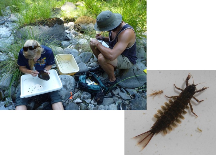 Epibenthic Invertebrates on cobbles (similar to Peggy’ Wilzbach’s rapid assessment method) Five cobbles are sampled along each transect–we choose cobbles that range from 60-120 mm median diameter, ~ grapefruit-sized stones. We use ~25 cm wide 1-mm mesh aquarium nets to sample epifaunal invertebrates on these coarse (large-pebble-large cobble) substrates. Placing the net downstream from the stone, we quickly roll the stone into the net and lift up so as to minimize loss of invertebrates. Then we brush off attached fauna into a white tray of water streamside. Bankside, seated next to a partner who records data, we first estimate the area of cobble sampled by measuring its major and minor axes (of the habitable area when rock was on the bed) and noting its shape (oval, rectangle, or triangle). These lengths will later be used to estimate habitable area. We then count numbers and estimated body lengths of every invertebrate 1 mm or larger) , keeping track of taxa at least to order, often to family, and sometimes to genus and species (see Appendix C for identification guide). Some invertebrates are measured within their cases, and this is noted. We have length-weight regressions for both invertebrate bodies, and invertebrate cases (the latter of course have much greater variation). Data on invertebrates are later entered into a controlled-vocabulary data base. We are happy to share this data base and its software with other users.
______________________________________________________________________________________________________________________________________________________________________________________________
Appendix A. Transect survey methods (MEP)
I repeatedly survey permanent cross-stream transects (“x-scns”) to follow changes in algae, environmental conditions, and associated organisms over time, documenting seasonal and interannual variation. Transects are benchmarked at both ends with nails in trees or bedrock—these can be labeled with aluminum tree tags (Forestry Supply) and should be carefully located with hand-drawn maps, GPS, triangulation (measure distance to spot from two other conspicuous landmarks), etc. Benchmarks should be on ‘permanent’ structures (e.g. large trunks) high enough so that high as well as low flows can be documented (just above bank full is ideal, higher than that and it’s hard to read the tape while walking the streambed). On each survey, stretch a meter tape tightly between the nails. Nail to nail distance should vary less than 1 cm over repeated surveys. Take enough points to obtain about 15-20 measurements for each x-scn. At 0.5 m or 1.0 m intervals along each transect:
- note distance along the meter tape (X-strm (m))
- measure water depth (cm) (a ski pole marked in decimeters is good, doesn’t flex in high flow, and saves you from falls)
- measure velocity with a current meter, or estimate surface current velocity (cm s-1) by timing floating objects across your measurement point1
- note dominant and subdominant substrate particle sizes2
- using a diving mask or plexiglass view box, note the dominant and subdominant macroscopic algal taxa within an estimated 10 cm x 10 cm area around each sampling point3
- record the modal height (cm) of attached filaments or the length from point of attachment of strands of algae floating over the site on the water surface, if these obscured view of the bed.
- characterize algal density (% cover) 4
- if possible (for Cladophora, zygnematales, perhaps Nostoc) characterize algal condition5
- note conspicuous animals within the same 100 cm2 observation area, bearing in mind that some will be attracted to you (minnows) and others will be hiding (mayflies). These opportunistic observations are not as consistent or important as more systematic data collected from cobble inspection and snorkeling and bankside observation.
Key–Codes and categories used
Flow velocity (cm s-1)
0 (silt settles vertically)
0-5
5-10
10-20
20-30
30-50
50-100
>100
Wentworth Particle size (median diameter, mm)
<<< 2 mm, not gritty = silt, mud M
< 2, gritty = sand S
2-8 = small gravel Gs
8-16 = large gravel Gl
16-32 = small pebbles Ps
32-64 = large pebbles Pl
64-256 = cobbles C
> 256 but discrete = boulder Bld
continuous = bedrock Br
Algal (etc.) codes
Clad Cladophora (note color as green G, yellow Y or Rust R)
Moug, Spg Mougeotia or Spirogyra (need to distinguish under scope)
Zyg Zygnema (more chatreuse than Spg or Moug, earlier in season)
diat sk diatom skin (gold, orange or yellow-brown) on rocks
bg sk dark or grey skin (often Phormidium, Tolypothrix or Scytonema)
Nos b Nostoc balls
Nos e Nostoc ears (colonized by Cricotopus midge larvae)
Riv Rivularia black freckles to larger circular spots or blotches
Anab deep turquoise Anabaena, loosely epiphytic on Clado
Phor Phormidium—dark brown epilithic cyanobacteria turf in riffle flow
Sedge dominant bunched graminoid along active channel is Carex nudata
Moss Fontinalis is long moss, other riverine mosses are mats < 3 cm high
Leaves: Terrestrial leaf litter
Algal density (~ % cover)
- a few filaments
- < 10% basal cover
- 10-50% basal cover
- 50-99% cover
- can’t see substrate through growth
Algal condition (can’t assess for many taxa)
- nearly detritus
- senescent, discolored, fragile and falling apart
- discolored but less fragile
- slightly discolored, but robust
- vibrantly healthy